Cool Cities Lab aims to provide city officials with necessary data and insights to optimize and accelerate the implementation of heat-resilient urban infrastructure solutions and reduce population exposure to extreme heat conditions in urban settings.

The application is designed for a primary audience of city officials sitting in departments concerned with urban planning and climate adaptation. It aims to support them in the following areas:

• Understanding their baseline heat risk and current heat-related infrastructure. Many of our users told us that information to characterize the nature of extreme heat locally is absent for their community.
• Assessing the spatial distribution across their city of heat-risk and risk-mitigation opportunities. Our users highlighted their need for methods to understand the spatial variation of relative risk from extreme heat and of opportunities to address it. For example, they lack evidence to identify priority plantable areas to maximize the benefits of their tree-planting programs.
• Accessing hyperlocal spatial and temporal estimates of thermal stress and air temperature that they can integrate in their urban plans and project documentation. Our users told us they lack access to open data providing heat mapping (especially for metrics of heat hazards most relevant to health: metrics related to thermal stress and air temperature) at high resolution in their cities to inform their planning decisions.
• Adopting a data-driven approach to selecting among heat-resilient infrastructure options. Our users lacked information on the local potential for implementing various solutions and the trade-offs between them.
• Estimating cooling impact and benefits of various passive cooling infrastructure solutions, including tree planting, reflective surfaces, and shade structures. Our users expressed the need for quantitative evidence of the potential cooling impact of planned heat-resilient infrastructure to unlock funding opportunities and influence decision-making.

Urban areas are often significantly hotter than surrounding rural regions and are warming at twice the global average rate (UNEP 2021). Yet the same characteristics that drive this heat—particularly dark, impervious surfaces and a lack of vegetation—also present opportunities for mitigation through thoughtful urban design. Heat-resilient infrastructure, such as trees, vegetation, cool roofs, and reflective pavements, can reduce individual heat exposure and lower area-wide temperatures when implemented at scale. And unlike active cooling infrastructure such as air conditioning, these passive solutions can also support cities in reaching net-zero energy goals.

Despite these benefits, cities often lack the information needed to identify the most effective heat-resilient interventions and where to implement them. Developing locally relevant analytical tools is frequently time-consuming, expensive, and out of reach for many urban decision-makers (Jain and Espey 2022). Additionally, insufficient capacity and expertise within city governments to obtain and refine vast quantities of data into actionable information and insights is a frequently reported challenge (Ukkusuri et al. 2024). While a core set of passive heat-mitigation strategies is widely recognized, the optimal combination of solutions is highly context-specific (UNEP 2021). Although more city plans are beginning to address urban heat, few include actionable data or a range of infrastructure solutions (Turner et al. 2022). Moreover, many existing data sources are not outcome-oriented enough to guide effective policy (Jain and Espey 2022).

To better understand cities’ needs related to long-term adaptation to rising temperatures and related infrastructure solutions, we conducted in-depth interviews and workshops with city officials, urban planners, and subject matter experts across South America, North America, Africa, South Asia, and Europe. These included city officials from Monterrey, Mexico; Rio de Janeiro, Brazil; Cape Town, South Africa; Dhaka North, Bangladesh; and Barcelona, Spain. In 2023, we engaged 12 subject matter experts and 40 potential data users; in 2024, this expanded to 27 experts and 170 potential data users, including engagements with participants at heat-focused workshops and in-person meetings and events. We used insights from these interviews, workshops, and surveys to inform the design of Cool Cities Lab and the analytical methods that power it.

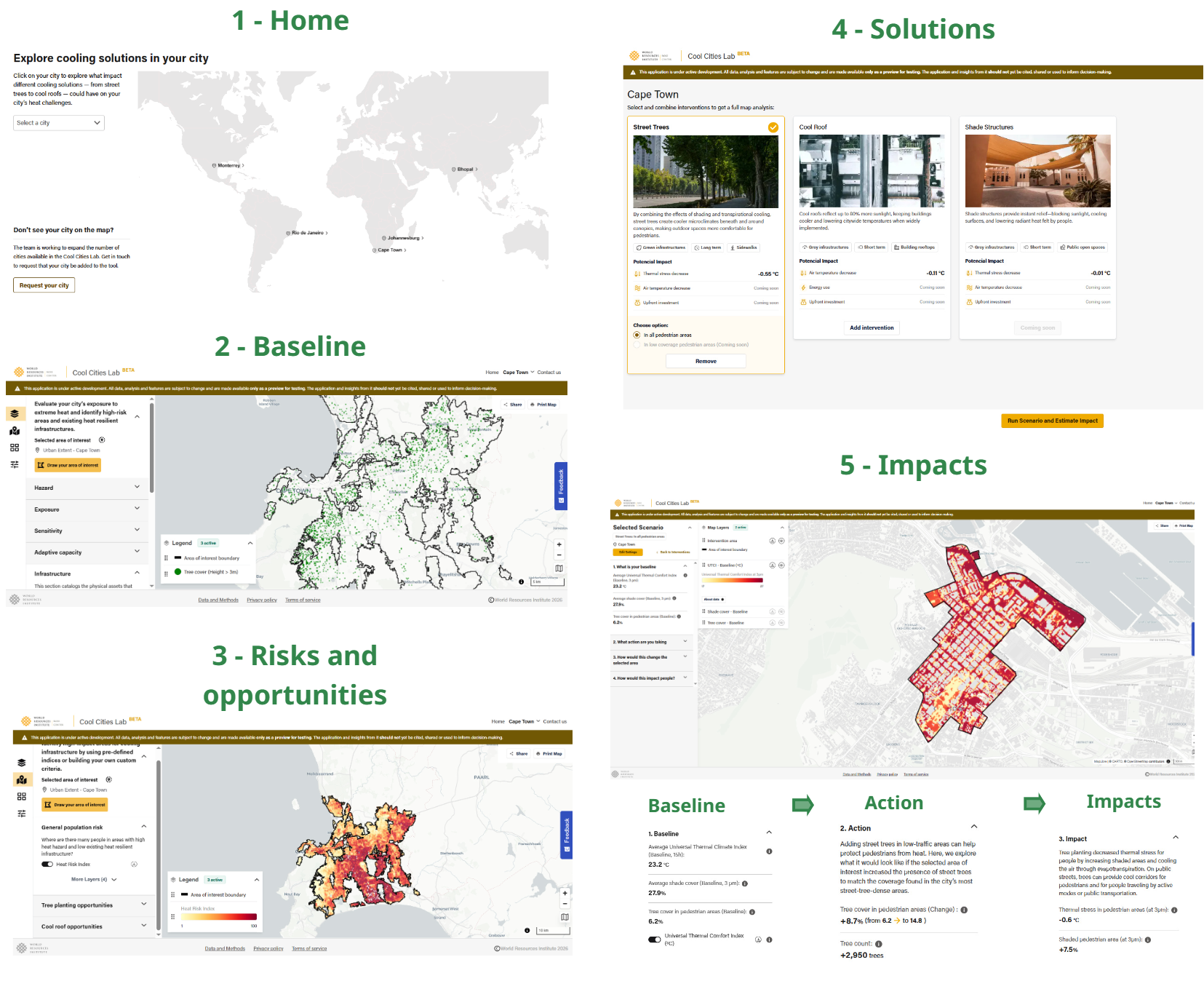
Cool Cities Lab is organized in seven main pages:

• Home: A landing page where you can learn about the main functionalities of the tool and select your city of interest.
• Baseline: Provides access to data layers and indicators for assessing baseline heat conditions in your city.
• Risks and opportunities: Provides access to heat risk indices to support prioritizing areas for heat action planning.
• Solutions: Presents the different cooling interventions modeled in the tool that you can select to explore potential impacts in your city.
• Impacts: Groups datasets, layers, and indicators available to explore and download to understand your city’s heat-resilience baseline and estimate the cooling potential of selected interventions.
• Contact us: A contact form where you can share a message or express a request to the Cool Cities Lab development team.
• Data and methods: Lists and documents the different datasets available in the application with the underlying methods.

The user flow is structured to select your city on the home page, explore contextual data about the city in the “Baseline” page, use the “Risks and opportunities” page to identify areas within the city on which to focus, select an intervention of interest in the “Solutions” page, which will drive you to the “Impacts” page, where you can browse and visualize relevant data layers and metrics related to the simulated impact of your selected intervention.

Home page

The home page is used as a landing page where you can access a summary description of the tool’s main functionalities and learn about the Data for Cool Cities initiative supporting the product’s development.

Two options are available for selecting your city:

• Using the drop-down list
• Selecting your city directly on the map, which will cause the name of the city to be highlighted with orange background

When you select your city, you will be directed automatically to the “Baseline” page. There you can explore various contextual datasets about heat risks and infrastructure in the city.

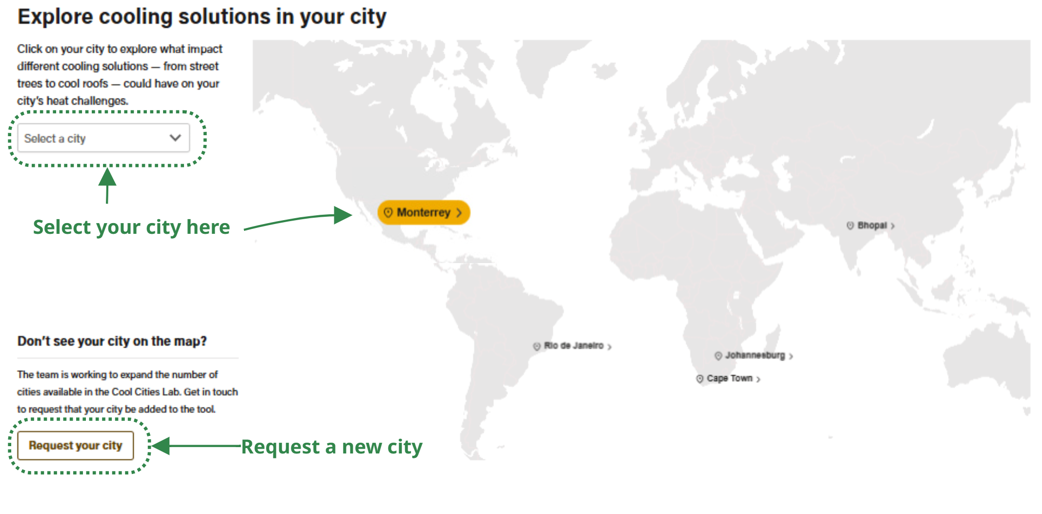
If your city is not available on the map and on the drop-down list, you can send a request to add your city by clicking on the button “Request your city.” This will direct you to a contact form to specify your request.

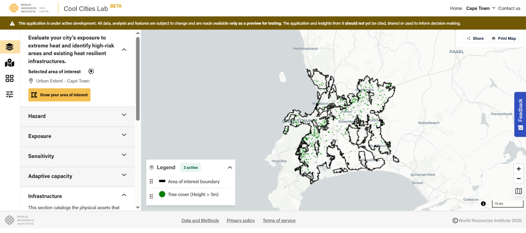
Baseline page

This page provides users with spatial data layers and indicators that measure key dimensions of the current state of heat hazard and heat-related infrastructure in an area of interest.

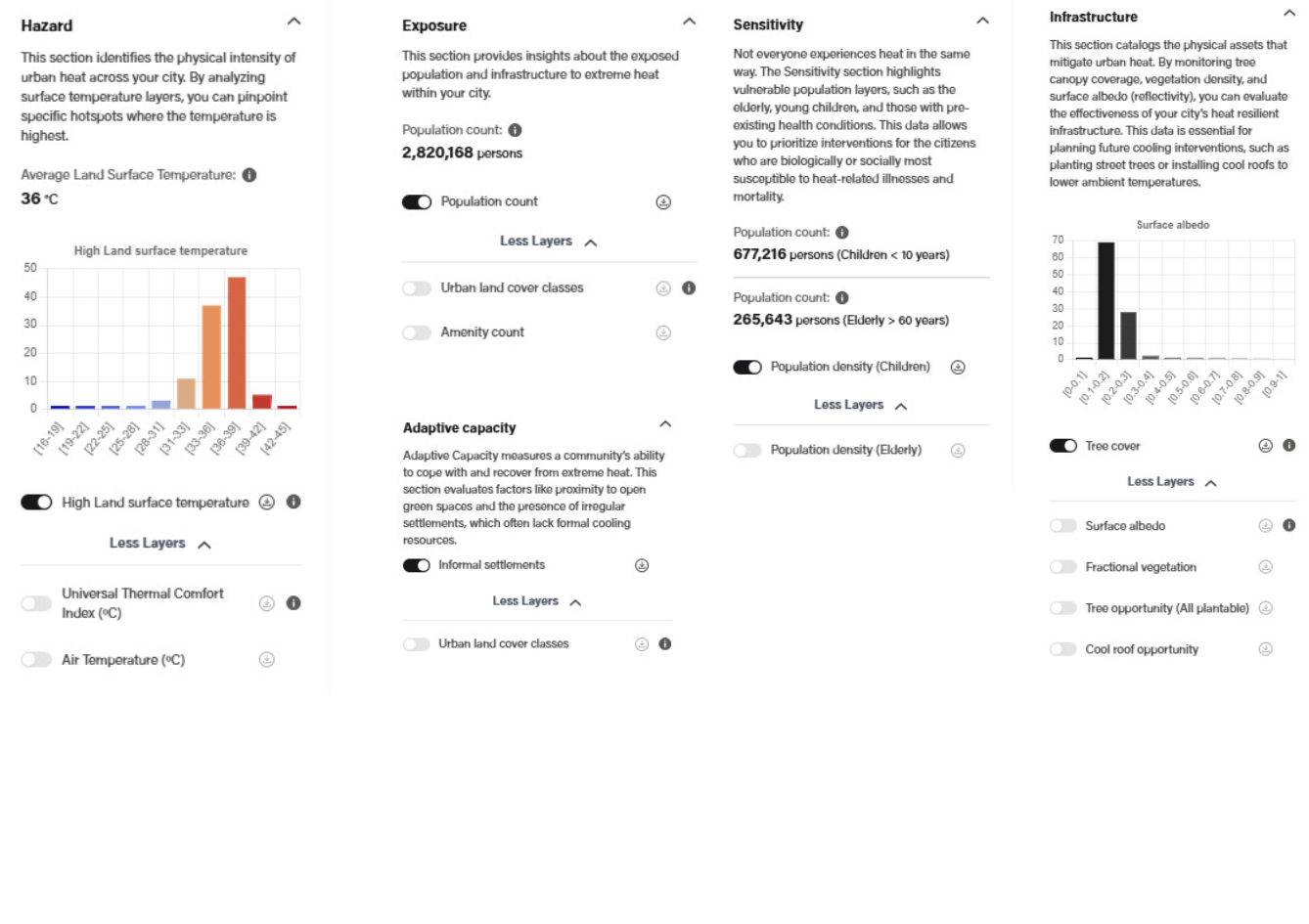
At the urban extent level or for a custom area of interest within an available urban area, users can browse maps, get summary statistics, and view charts for assessing key dimensions for heat risk assessment organized in five subsections: Hazard, Exposure, Sensitivity, Adaptive capacity, and Infrastructure. Every section compiles a list of data layers, summary indicators, and charts for assessing baseline conditions.

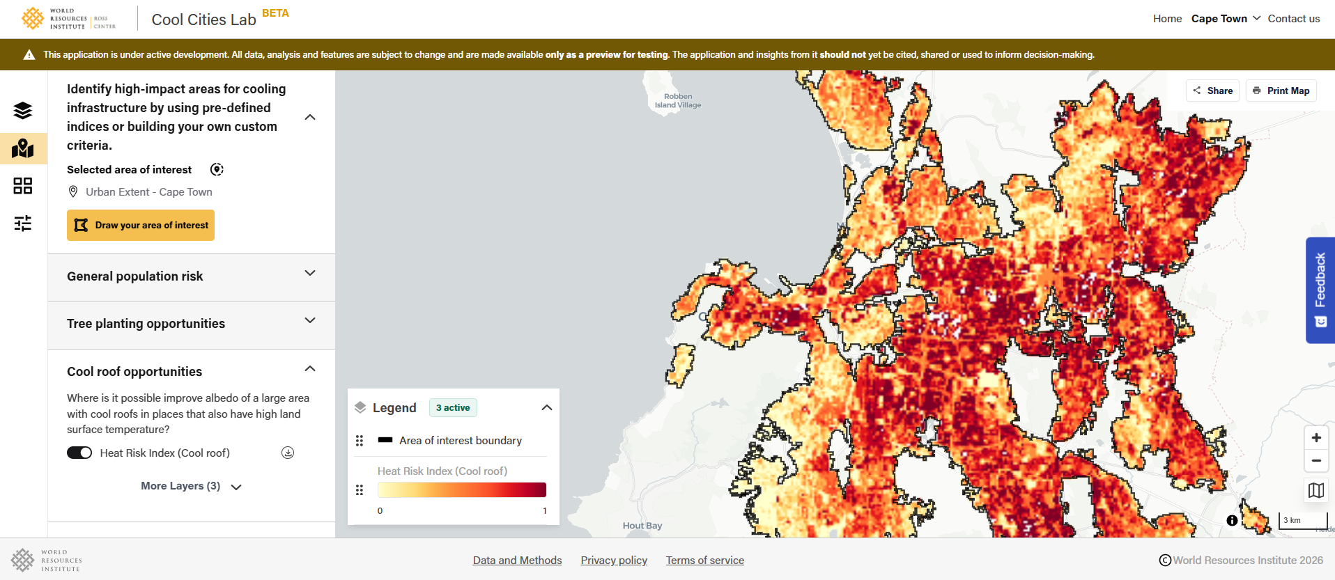
Risks and opportunities page

This page provides a list of spatial heat risk and opportunities indices calculated from datasets available on the Baseline page. Three predefined spatial indices are available in Cool Cities Lab for all included cities and can be used to identify areas within an urban area that have higher risk from extreme heat and/or that have higher opportunity for implementation of cooling infrastructure.

• General population risk index: This index helps identify priority sites where there are many people in areas with high heat hazard and low existing heat-resilient infrastructure.
• Priority tree opportunity index: This index helps identify priority sites where it is possible to plant many trees in places that also have high temperature and high amenity density.
• Priority cool roof opportunity index: This index helps identify priority sites where it is possible to improve albedo of a large area with cool roofs in places that also have high land surface temperature.

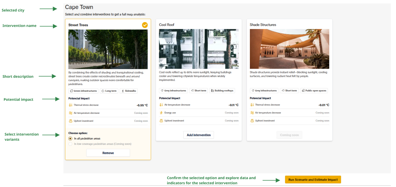
Solutions page

Once you select your city, you will be invited to select a heat-resilience intervention of interest to explore simulated results of implementing it in a specific area of interest in your city. The Solutions and Impacts pages are not available for every city.

Three types of solutions are available in Cool Cities Lab: street trees, cool roofs, and shade structures. You can select the intervention of interest by clicking on the “Add intervention” button within the specific card. You can then select a variant of the selected intervention based on the available options that will appear once you have selected your intervention. For example, if you choose “Street trees,” you can select between two options: planting trees in all pedestrian areas (with no prioritization criteria) or focusing only on areas within your city with low tree cover.

You can also select a scenario combining multiple interventions, only available for some cities and for combining “Street trees” with “Cool roofs” in the current release. When you select the “Street trees” intervention, you can add “Cool roofs” to explore a scenario showing a combined effect of both interventions in your city.

The intervention cards provide summary information about the modeled heat-resilience interventions with a short description, as well as their potential impact in terms of thermal stress and air temperature decrease.

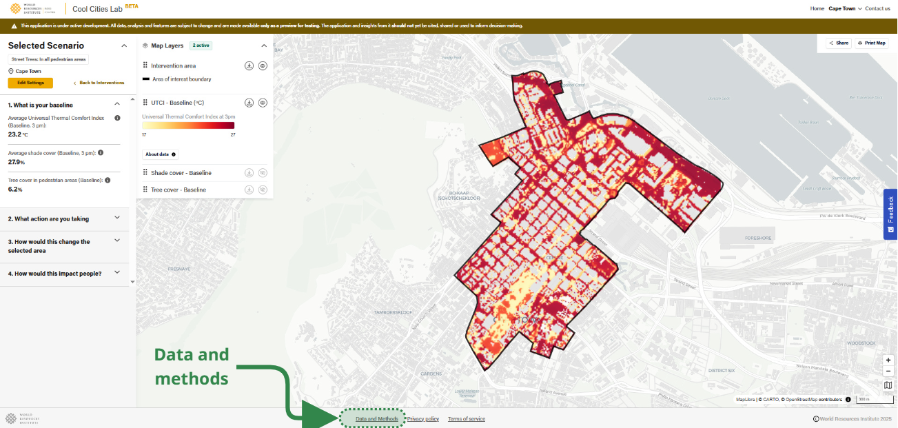
Impacts page

When you select an intervention you will be directed to the “Impacts” page, where you can access, explore, and download all data relevant to assessing heat exposure in your city, identify areas where the selected intervention could be implemented, and explore the cooling impact of a predefined scenario modeled in your area of interest.

The “Impacts” page offers various functionalities to explore and interact with the data layers and indicators produced to simulate the cooling impact of selected interventions.

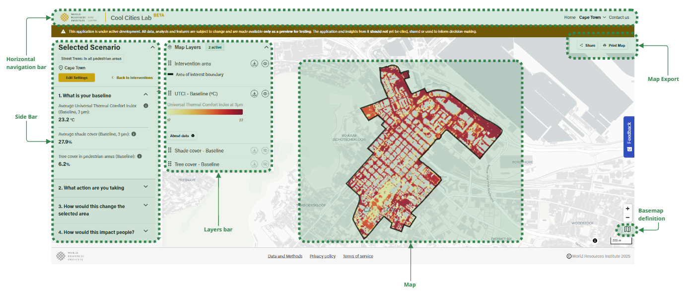
The page is organized in three successive sections to guide you through the different steps to understand the heat exposure baseline and the cooling potential of the simulated scenario. Every section is connected to a list of indicators and data layers that will appear in the tool once you click on the title to unfold it. We encourage you to follow the order of the sections to assimilate the complete narrative, from baseline to cooling impact assessment. Not all indicators and data layers are available for every city.

1. Baseline

This subsection provides a list of indicators, or summary statistics, and data layers to understand baseline conditions of heat exposure and resilience in your city that are relevant for a selected intervention and area of interest.

Selected intervention	Street trees	Cool roofs	Shade structures in parks
Indicators	Air temperature at 3 p.m. (in outdoor areas, °C) Thermal stress at 3 p.m. (in pedestrian areas, °C universal thermal climate index [UTCI]) Thermal stress category at 3 p.m. (in pedestrian areas, % "strong" or worse) Shade cover at 3 p.m. (in pedestrian areas, %) Tree cover (in pedestrian areas, %)	Air temperature at 3 p.m. (in outdoor areas, °C) Roof reflectivity (albedo)	Thermal stress at 3 p.m. (in parks, °C UTCI) Thermal stress category at 3 p.m. (in parks, % "strong" or worse) Shade cover at 3 p.m. (in parks, %) Distance to shade at 3 p.m. (in parks, meters)
Layers	Air temperature—baseline at 3 p.m. (°C) Thermal stress—baseline at 3 p.m. (°C UTCI) Thermal stress—baseline at 3 p.m. (categories) Shade cover—baseline at 3 p.m. Tree cover—baseline	Air temperature—baseline at 3 p.m. (°C) Roof reflectivity—baseline (albedo)	Parks Thermal stress—baseline at 3 p.m. (°C UTCI) Thermal stress—baseline at 3 p.m. (categories) Shade cover—baseline at 3 p.m. Distance to shade—baseline at 3 p.m. (meters)

2. Action

This subsection provides a list of summary statistics and data layers to explore the intervention simulated in your city. The simulation is parametrized to achieve a realistic target, based on data for your city.

Selected intervention	Street trees	Cool roofs	Shade structures in parks
Indicators	Tree cover—achievable target (in pedestrian areas, %) Tree cover—change (in pedestrian areas, %) Tree count—change (#)	Roof reflectivity—achievable target (albedo) Roof reflectivity—change (albedo) Area of cool roofs (m2)	Shade cover—change at 3 p.m. (in parks, %) Shade structure count—change (#)
Layers	Tree cover—change Tree cover—scenario Plantable areas Pedestrian areas	Roof reflectivity—change (albedo) Roof reflectivity—scenario (albedo)	Shade structures Parks Shade cover—change Shade cover—scenario

3. Impacts

This subsection provides a list of indicators, or summary statistics, and data layers to understand the impacts, or results, customized to the city, of implementing the scenario defined in the “Action” subsection.

Selected intervention	Street trees	Cool roofs	Shade structures in parks
Indicators	Air temperature—change at 3 p.m. (°C) Thermal stress—change at 3 p.m. (in pedestrian areas, °C universal thermal climate index [UTCI]) Shade cover at 3 p.m. (in pedestrian areas, %)	Air temperature—change at 3 p.m. (°C) Thermal stress—change at 3 p.m. (in outdoor areas, °C UTCI)	Thermal stress—change at 3 p.m. (in parks, °C UTCI) Shade cover at 3 p.m. (in parks, %) Distance to shade at 3 p.m. (in parks, meters)
Charts	Air temperature (°C) Thermal stress (in pedestrian areas, °C UTCI) Shade cover (in pedestrian areas, %)	Air temperature (°C)	Thermal stress (in parks, °C UTCI) Shade cover (in parks, %)
Layers	Air temperature—change (°C) Thermal stress—change (°C UTCI) Thermal stress—change (categories) Shade cover—change Air temperature—scenario (°C) Thermal stress—scenario (°C UTCI) Thermal stress—scenario (categories) Shade cover—scenario	Air temperature—change (°C) Thermal stress—change (°C UTCI) Air temperature—scenario (°C) Thermal stress—scenario (°C UTCI)	Thermal stress—change (°C UTCI) Thermal stress—change (categories) Shade cover—change (%) Distance to shade—change (meters) Thermal stress—scenario (°C UTCI) Thermal stress—scenario (categories) Shade cover—scenario (%) Distance to shade—scenario at 3 p.m. (meters)

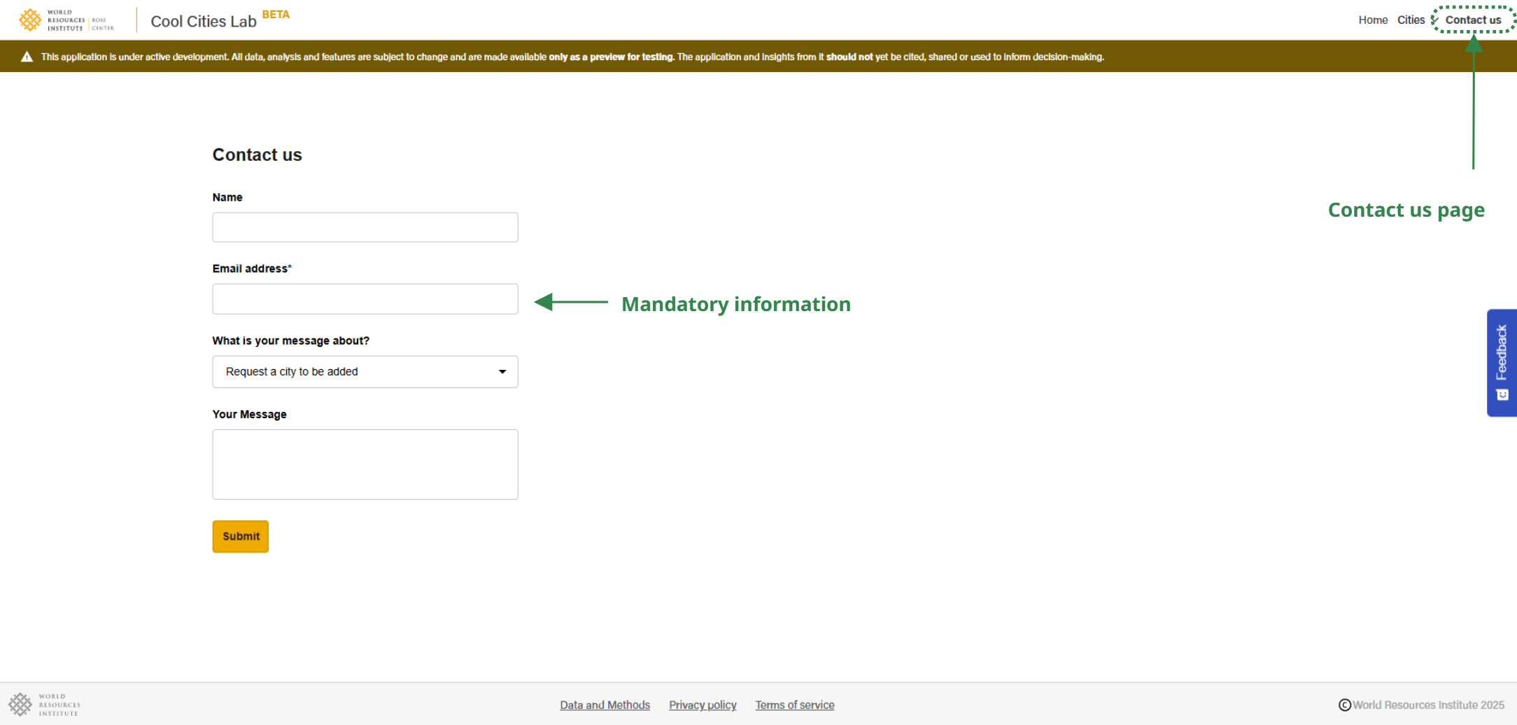
Contact us page

This page provides a form that you can use to contact us directly by expressing specific requests: to add your city to the platform, to add a new intervention to our model, or to share with us a general feedback or inquiry. This page is accessible either directly by clicking on “Contact us” in the horizontal bar or by clicking on “Request your city” on the Home page.

On this contact form, you can specify your name, your email address, the type of request among a predefined list, and a message. Our team will aim to respond using the email address you provide in order to learn more about your request and help you use Cool Cities Lab.

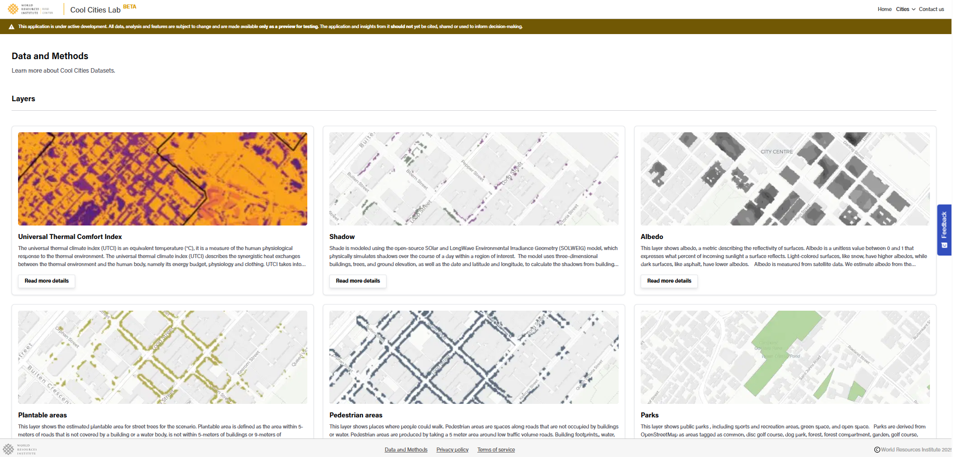
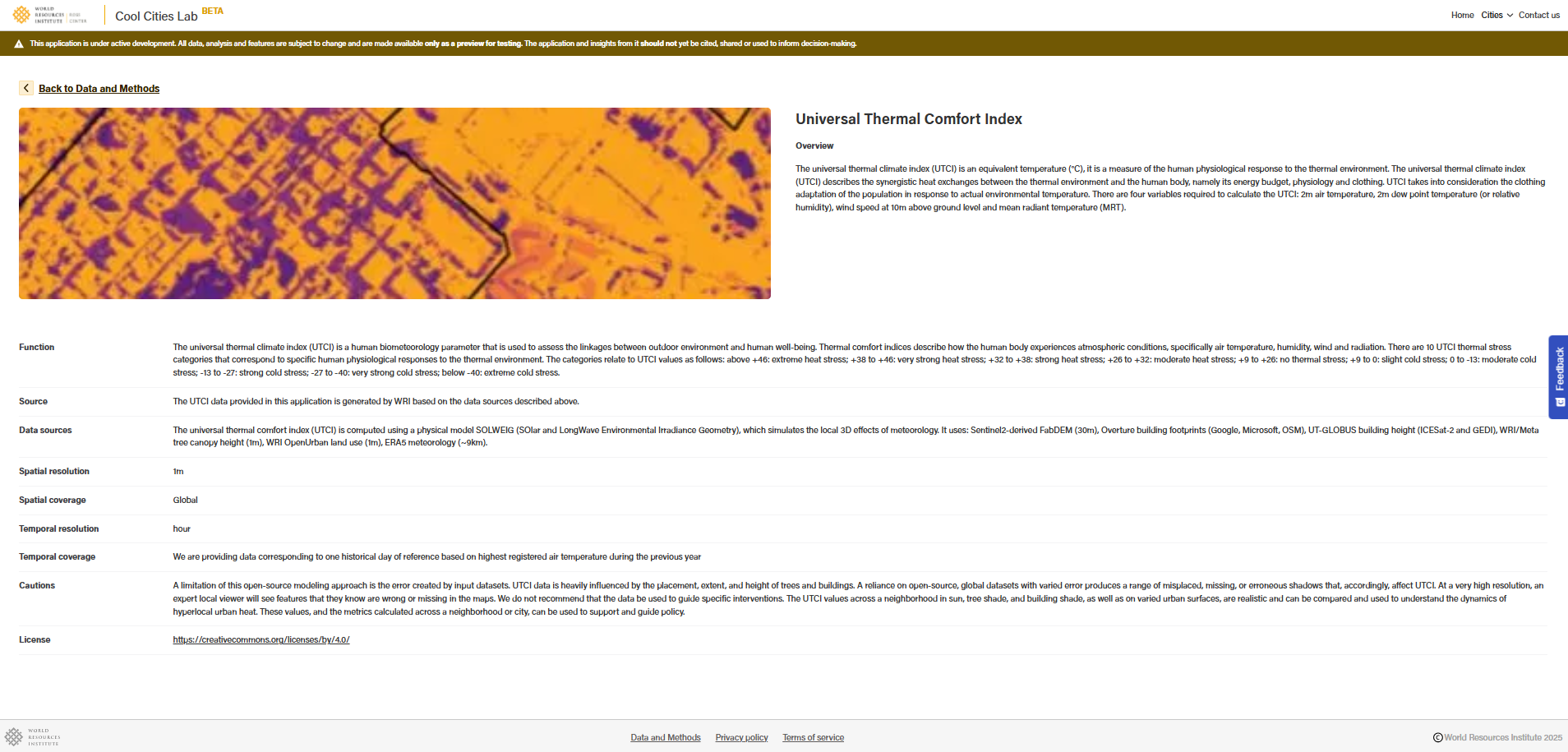
Data and methods page

This page, which is accessible from the bottom horizontal bar, contains documentation of the methods used to produce the data and indicators available in the platform. Every dataset is represented on a separate card. When you click on it, a page with metadata describing the method used to produce the data layers will appear, including the following information: overview, function, source, data sources, spatial resolution, spatial coverage, temporal resolution, temporal coverage, cautions, and license.

Data exploration components

Common navigation features found throughout the site are described in more detail below.

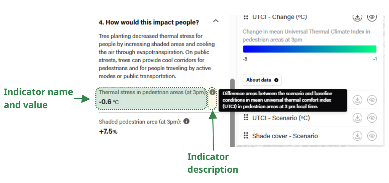
Indicator component

For every indicator in the sidebar, you can find the associated value and unit. By hovering over the “information” icon, you can access a definition of the indicator.

Layer selection component

Near each indicator there is also an option to interact with the related layer on the map. When you select a section in the sidebar, the layers bar will update automatically and show a list of layers relevant for the selected section. Some layers are turned on and visible by default, while others are turned off. For each available layer there are three icons:

• A “Show/hide” toggle button () icon to turn the layer on or off.
• A “Download” icon () for downloading the used dataset (in geotif format for raster data and geojson format for vector data).
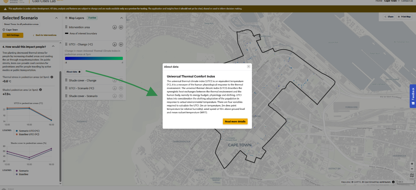
• An “About data” icon () to read more details about the method used for producing the data layer. When you click on this button, a “window panel” will open describing the method for calculating the layer. It will also offer the possibility of reading a longer version of the layer’s metadata by clicking on “Read more details.”

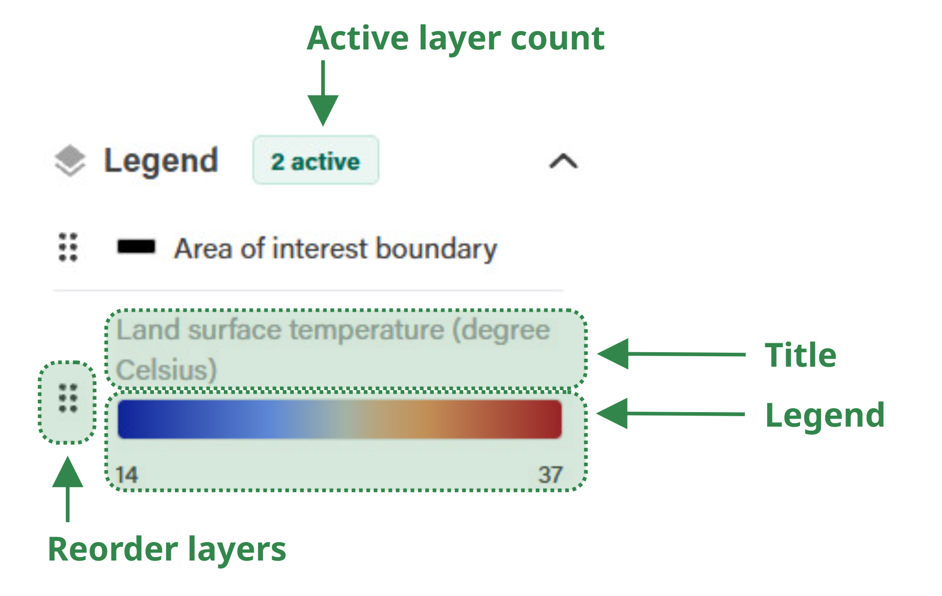
Legend box

The legend box provides information on the number and meaning of the layers currently visualized in the map. Every layer is characterized by

• a title;
• a legend describing the meaning of the iconography or colors used; and
• a reorder icon () to change the order of the layer in the layer stack.

Legend box

Layer: About data functionality

Map

You can explore the different data layers available in the layers bar interactively on the map. All the turned-on layers are stacked on the map following the order in the layers bar. The layers are also cropped to show data only in the area of interest.

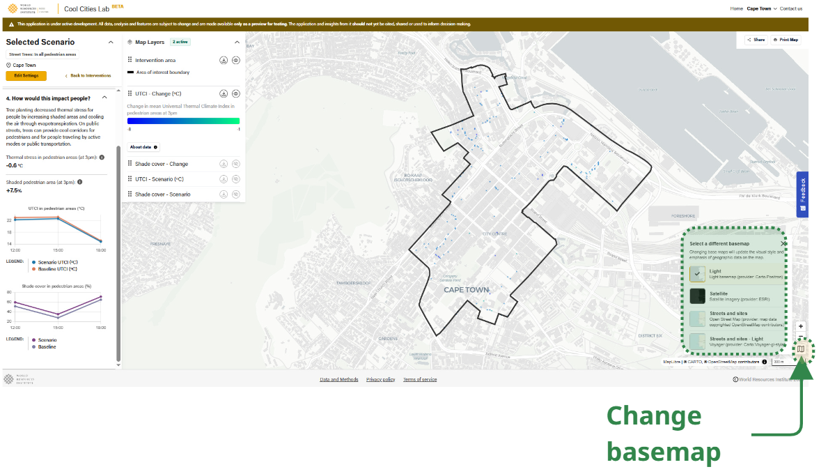
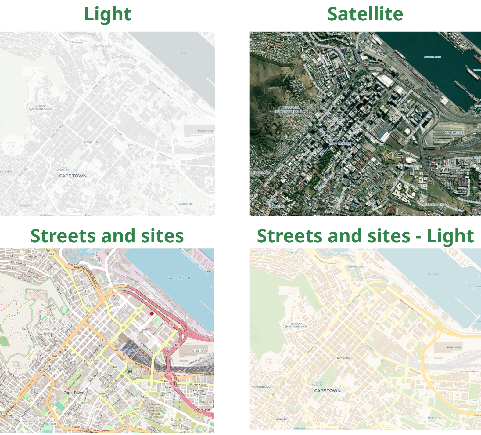
Basemap

You can change the basemap by clicking on the basemap icon. Four types of baseline are available in Cool Cities Lab: Light (source: Carto Positron), Satellite (source: Esri), Streets and sites (source: OpenStreetMap), Streets and sites light (source: Carto Voyager).

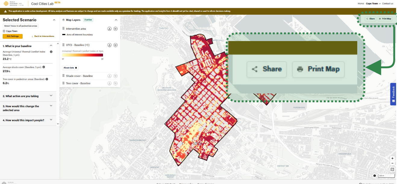
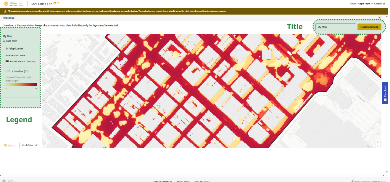
Print map

The functionality “Print map” allows you to export the map with the same parameters that you defined in the tool (zoom level, zoom area, layers order) as a pdf file to print it or integrate it into other documents.

When you click on “Print map,” a window will appear showing a ready-to-print view of the map with the associated legend. You can add a title and save the map as a pdf file on your device.

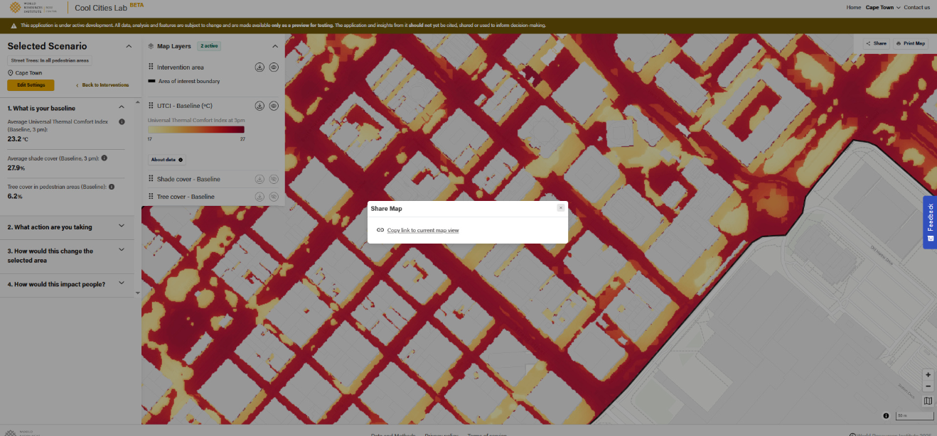
Share map

When you click on “Share map,” a panel window will appear to copy a URL that you can use to share the exact same view that you are exploring with others.

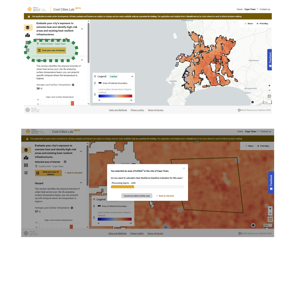
Custom area of interest

You can calculate indicators based on a custom area of interest that you draw in Cool Cities Lab. By clicking on “Draw your area of interest,” you can define a polygon and run zonal statistics live in the tool to generate indicators based on the defined polygon. After confirming the analysis, the indicators in the sidebar will be updated based on the new polygon area.

The datasets and methods used in Cool Cities Lab are pulled from many sources. This section is intended to provide a general overview of the methods used, describe how they interact with each other, and point to documents that provide additional details on specific elements. A summary of the methodological elements is included in the graphic below. Methods described in this document are in green. Methods documented in other publications are in other colors.

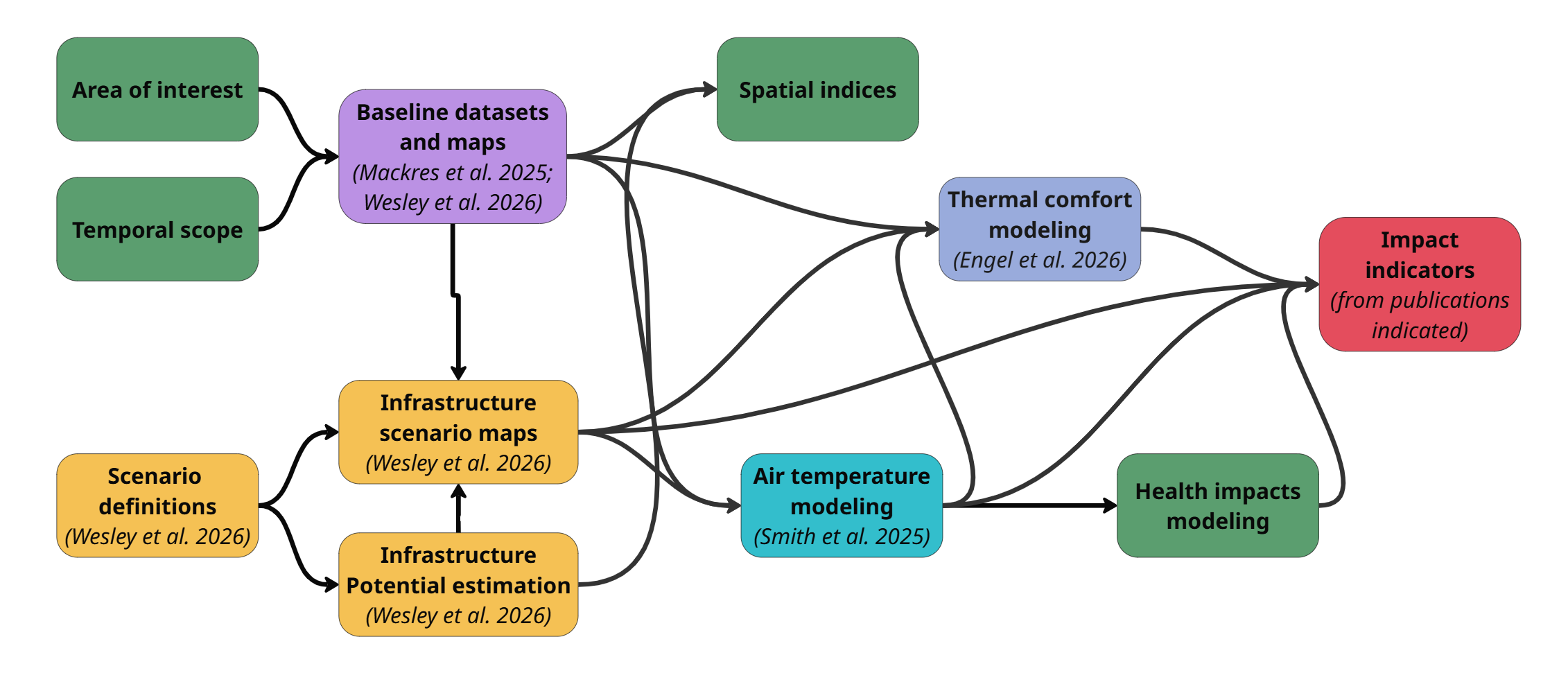
Source: WRI authors.

Areas of interest

Users can select an area of interest from within any urban area included in the tool. The urban areas included in the tool are based on requests from stakeholders in those locations and the availability of resources to generate the requisite data. By default, the area of interest for all urban areas is its urban extent, as defined by Angel et al. (2024). If a user is interested in a smaller area of interest within the larger urban area—such as a municipality, neighborhood, or corridor—they may draw or upload a polygon. The selected area of interest becomes the primary unit of analysis used by all other features in the tool, including generating summary indicators. Not all data may be available for the full urban extent area of interest. In particular, due to the significant computing resources required to produce them, thermal comfort layers are usually only available for a specific neighborhood or other small, subcity area of interest.

Temporal scope

Individual datasets, and sometime individual data points, used within Cool Cities Lab provide measurement from different time periods. In general, we aim to include baseline datasets that have the most recent information as well as the spatial resolutions and other characteristics required for our analyses.

When modeling heat impacts, we use a local extreme heat event from the recent past. This enables users to compare an estimate of the heat hazard experienced during that event based on current infrastructure with the hazard that would have been experienced if alternative infrastructure had been in place. This “alternative past” approach both helps to make the results more tangible to stakeholders (“Wouldn’t it have been nice if it had been two degrees cooler during the heat wave in August last year?”) and provides a conservative estimate grounded in an common experience that does not require understanding of or agreement on future local heat hazards in a changing climate.

Baseline

This feature provides users with spatial data layers and indicators that measure key dimensions of the current state of heat hazard and heat-related infrastructure in an area of interest.

For a custom area of interest within an available urban area, users can browse maps, get summary statistics and view charts on the following criteria:

• Tree cover
• Vegetation cover
• Surface albedo
• Land surface temperature
• Land cover classes
• Tree cover, vegetation, albedo, land surface temperature, shade cover, universal thermal climate index [UTCI] disaggregated by land cover classes
• Air temperature (where calculated)
• Shade cover (where calculated)
• Thermal stress (UTCI) (where calculated)
• Population by age and gender
• Seasonal temperature patterns (citywide, no map)
• Future heat hazards—expected number of heatwaves (citywide, no map)

These baseline statistics can be used as benchmarks from which to monitor progress or set targets for improvement or to enable spatial comparisons between city neighborhoods or between peer cities.

The data layers used for the baseline are from the same sources and methods as those used in other features of the tool, as documented in Wesley et al. (2026), Mackres et al. (2025), and Engel et al. (2026).

Spatial indices

This feature consists of map overlays and raster indices calculated from datasets provided for the baseline feature. Users can either select from predefined index options available with a single click and designed to answer common heat planning questions, or develop their own custom indices within the tool using the available datasets to answer locally relevant questions. The generated indices can be used to identify areas within an urban area that have higher risk from extreme heat and/or that have higher opportunity for implementation of cooling infrastructure. The index methods are built upon the heat vulnerability index literature (NASA Applied Sciences 2022; Gamble et al. 2018; Conlon et al. 2020; Qian and Liu 2025).

The custom spatial index feature includes the following index component categories and datasets (as well as their sources and methods):

• Hazard:
  • Universal Thermal Comfort Index (Engel et al. 2026; 1 m, custom date)
  • [Absence of] Shade (Engel et al. 2026; 1 m, custom date)
  • Air temperature (Smith et al. 2025; 100 m, custom date based on recent local extreme heat event)
  • Land surface temperature (Wesley et al. 2026; 30 m, custom date based on recent local extreme heat event)
• Exposure:
  • Population density (WorldPop in Mackres et al. 2025; 100 m, 2020)
  • Business density (OpenStreetMap in Mackres et al. 2025; vector to 100 meter (m) raster, most recent available data)
  • Amenity density (schools, health facilities, public transport) (OpenStreetMap in Mackres et al. 2025; vector to 100 m raster, most recent available data)
• Sensitivity:
  • Elderly, young children, women of childbearing age (WorldPop in Mackres et al. 2025; 100 m, 2020)
• Adaptivity capacity (change to directionality noted where lower values indicate higher risk):
  • Informal, irregular, or slum settlements (GIULU [Global Intra-urban Land Use] in Guzder-Williams et al. 2023; Mackres et al. 2025); 5 m, 2020)
  • [Low] Proximity to public open space (OpenStreetMap in Mackres et al. 2025; 100 m, most recent available data)
  • [Lack of] Tree cover (Tolan et al. 2024; Wesley et al. 2026; 1 m, 2020)
  • [Lack of] Vegetation (Wesley et al. 2026; 10 m, custom date)
  • [Low] Albedo (Wesley et al. 2026; 10 m, custom date)
  • [Lack of] Shade (Engel et al. 2026; 1 m, custom date)
• Infrastructure opportunity:
  • Tree opportunity (Wesley et al. 2026; 100 m, 2020)
  • Cool roof opportunity (Wesley et al. 2026; 100 m, custom date)

Not all datasets may be available for every city. Each dataset has uses that are more or less appropriate in a spatial index depending on the objectives of each user. In the tool, index dataset options are accompanied by cautions and guidance on their recommended uses. For example, land surface temperature is a poor indicator for human exposure to heat hazards, but it is more appropriate indicator for measuring the hazard to infrastructure.

All included datasets are available for viewing as layers in the application at their native resolution and units. They will also be further processed to enable them to be used to create a user-customized spatial index layer using a variation on the “ecological method” (McHarg 1969). Including both the source data and derived indices as layers in the same viewer allows users to visually assess the contributions of each selected layer to their generated index.

For the index, all datasets are aggregated to a common raster resolution based on the lowest-resolution dataset (100 m, to match WorldPop) and then resampled to align all datasets to a common raster grid (WorldPop is used as the reference grid). Custom spatial, raster-based indices will be calculated based on user-selected layers and weights. Both predefined and custom indices are generated “on the fly” in the application based on user selections.

Predefined indices include the following:

• General population risk: Where are there many people in areas with high heat hazard and low existing heat-resilient infrastructure?
  • Hazard: air temperature (or, if not available, land surface temperature)
  • Exposure: population density
  • Existing infrastructure: open spaces, tree cover, vegetation, albedo
• Priority cool roof opportunity: Where is it possible improve albedo of a large area with cool roofs in places that also have high land surface temperature?
  • Hazard: land surface temperature
  • Opportunity: cool roof opportunity
• Priority tree opportunity: Where is it possible to plant many trees in places that also have high ground-level thermal stress and high amenity density (a proxy for pedestrian activity)?
  • Hazard: Universal Thermal Comfort Index
  • Opportunity: tree cover opportunity
  • Exposure: amenity density

Here are two potential custom indices:

• A user interested in identifying city areas that currently have low tree cover but high tree cover opportunity could select only these two layers.
• A user interested in a heat risk index based on the exposure of elderly people at public transport stops to high ambient temperatures could select air temperature as the hazard, public transport density as the exposure, and elderly population as the sensitivity.

Each selected component category is given equal weight in the final index to reduce the risk of autocorrelation between datasets within a component category (for example, there is often a higher business density in areas of higher population density, which demonstrates that these two exposure variables are related and their effects on the index would be amplified if both were included without accounting for their relationship). However, if a user selects more than one dataset in a category, they can customize the weight given to each dataset (e.g., in the exposure category, if both population density and business density were selected they would by default each get 50 percent of the weight for that category, but the user could customize this to an 80/20 distribution of the weight).

The index calculation process includes six steps:

1. When relevant, normalize all factors into proportions (e.g., population over 65 / total population).
2. Ensure unidirectionally of factors: higher values should mean higher risk or opportunity.
3. Normalize by converting the dataset values of each factor within the area of interest into percentile-rank values from 0 to 1 (Price et al. 2025; Flanagan et al. n.d.). We use this approach, rather than standardization (Mallen et al. 2019; Reid et al. 2009), because many of the datasets we are working with have skewed distributions or outliers and because for our purposes it is more important to understand which areas are relatively higher or lower in risk than to highlight the magnitude of difference between them (Esri 2024, n.d.).
4. If multiple factors or datasets are included within a component, to maintain equal weight between components, assign weights within the component to each dataset prior to summing. For example, giving 80 percent of the weight to dataset 1 and the remainder to dataset 2 (notated as D1 and D2): (D1 * 0.8) + (D2 * 0.2)).
5. Sum the values of all components and convert the resulting sums to percentile-rank values from 0 to 1 to create the final index.
6. Categorize index values into five equally sized bins, or quintiles, ensuring a middle “average conditions” category.

Infrastructure scenarios

The infrastructure scenario feature of Cool Cities Lab allows users to select from multiple precalculated spatial implementation scenarios related to increased vegetation and tree cover, surface reflectivity, and shade. The methods used to develop these spatial scenarios are further detailed in Wesley et al. (2026).

Thermal comfort modeling

Cool Cities Lab can estimate the thermal comfort and stress impacts of meteorological and urban infrastructure scenarios at high spatial resolution, which allows for the comparison of the thermal stress impacts of multiple scenarios. These calculations use as inputs the datasets described in Wesley et al. (2026) and the modeling methods further detailed in Engel et al. (2026).

Air temperature modeling

Cool Cities Lab also provides estimates of intraurban air temperature effects of infrastructure changes. The methods behind these calculations for the New England region are further detailed in Smith et al. (2025). These methods are currently being generalized to enable air temperature inferences for additional regions.

Health impact modeling

To estimate the health impacts of extreme temperatures and the health effects of changes to temperature, we use the literature on city- and region-specific exposure-response relationships between air temperature and mortality (Gasparrini et al. 2015; Vicedo-Cabrera et al. 2019; Zhao et al. 2021; Kephart et al. 2022; Bakhtsiyarava et al. 2025). These epidemiological studies compare the statistical relationship between daily mean air temperature and daily death statistics to establish relative risk curves that present the risk of mortality in that city at specific temperatures relative to the risk at the temperature of minimum mortality (MMT) specific to that city. The result is an estimate of the excess deaths due to nonoptimal temperature, if compared to a hypothetical situation in which temperature is constantly equal to the MMT.

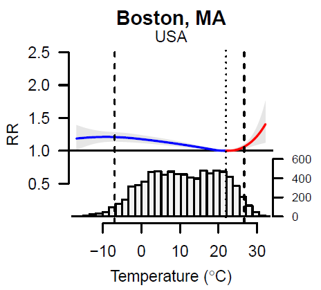
Source: Gasparrini et al. 2015.

We use these relative risk curves to calculate estimated mortality impacts of specific temperatures, and those resulting from changes to temperatures as estimated thorough air temperature effects modeling. Because we rely on the relationships established in these studies, we are only able to produce impacts of mortality estimates for cities and regions where this research has been completed. We currently lack access to the underlying data upon which these curve figures are based, so we reconstruct equations from the published figures by extracting sample points and using polynomial approximation with a best-fit curve calculator (graphreader.com 2023; Standards Applied 2024). Future work will aim to get access to the underlying data and, in cases where that is not possible, automate the curve-fitting methods.

First, we calculate the population-weighted mean daily air temperature for the scenario of interest. We estimate the mean from the average of the minimum and maximum temperatures, a simple, well-established method that also allows us to use minimum temperature values derived from one source and maximum temperature values derived from the same source but further processed for use in a temperature effects model at higher resolution (Bernhardt et al. 2018; Smith et al. 2025).

• Minimum: minimum air temperature from Daymet or ERA5-Land
• Maximum: air temperature at 3 p.m. from Smith et al. (2025), using only land areas overlapping with the minimum air temperature (ERA5-Land is missing land area in pixels that include water)

Unfortunately, Smith et al. (2025) is only appropriate for daytime temperatures, which requires us to use different methods to obtain the minimum and maximum temperatures. Regional datasets like Daymet and ERA5-Land have known limitations in their representation of urban microclimates, as they do not effectively account for the urban heat-island effect. As a result, our methods may systematically underestimate mean air temperatures, resulting in conservative estimates of health effects.

We add population weighting to each temperature raster using the WorldPop 100 m gridded population product (“WorldPop: Population Counts” n.d.). Finally, we average the minimum and maximum values to estimate the daily mean.

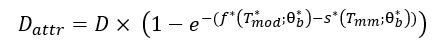
To calculate the estimated attributable mortality fraction from temperature, we use the population-weighted daily mean temperature to solve for the associated relative risk of mortality based on the established curve for the city or region of interest. For example, for Boston, the exposure-response curve per Gasparrini et al. (2015), extracted from the published figure as a best-fit curve, is represented by the equation

with x representing the daily mean air temperature and y representing the mortality risk relative to the MMT. The attributable mortality fraction is y – 1. In Boston, a temperature of 30 degrees Celsius, for example, corresponds to an attributable mortality fraction of 24.7 percent. We present the estimated attributable mortality fraction and 95 percent empirical confidence intervals.

Finally, to calculate estimated attributable deaths from cumulative, lagging temperature effects in the 21 days following a heat event, similar to Mistry and Gasparrini (2024) and Takacs et al. (2025) but instead focused on single heat events, we multiply the local crude death rate per day by the total population of the location of interest, then multiply by the attributable mortality fraction divided by the relative risk. By using cumulative exposure-response relationships integrated over a 21-day lag period, these estimates account for mortality displacement (harvesting) and represent net excess deaths rather than acute effects alone. Using annual crude death rates assumes uniform mortality throughout the year. We are limited to this assumption by the available data, but development of datasets on local seasonal variations in mortality is an opportunity for future research. As our research is focused on estimates for specific heat events, we do not attempt to quantify total annual mortality effects, nor do we address the effects of cold on mortality.

As an example, based on an annual crude death rate of 898 per 100,000 people in Massachusetts (and total population of 675,000 for the city of Boston), one day with a mean temperature of 30 degrees Celsius (a temperature that has a cumulative relative risk of death of 1.247) in Boston would be associated with 3.29 attributable deaths in the city (Massachusetts Department of Public Health 2023; US Census n.d.). The formula for this calculation, per Equation 2 of Vicedo-Cabrera et al. (2019), is

which simplifies to

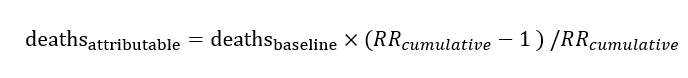
The calculation for the Boston example described is


To compare between two or more scenarios of interest, we take the difference between the attributable mortality fractions and attributable deaths calculated in each scenario to estimate marginal lives saved or lost as a result of the temperature change that results from the infrastructure scenario.

Cool Cities Lab can be applied to produce, for any city in the world, quantified estimates of heat effects of infrastructure changes. This is a major contribution to applied science of heat-resilience planning, providing new evidence to bolster the case for urban adaptation action. However, as with any research, there is uncertainty associated with the results, limitations on how the results should be interpreted, and cautions on how they should be used. Users should understand several limitations:

• Global datasets have inaccuracies and imprecision. The scalability of Cool Cities Lab is the result of a reliance on globally available datasets. The data required to do our analyses are available or can be produced for any city in the world—a major advantage of our approach. However, there are also disadvantages to using global datasets. Primarily, they may be inferior to alternative locally or nationally available datasets in accuracy, recency, official status, or other dimensions of importance to the users of Cool Cities Lab and their stakeholders. If there are no alternative local datasets this is not a concern—analysis based on global data is better than none at all. But even in these contexts, users should be aware that the data used in the analysis may be incomplete, inaccurate, or otherwise not fully reflect the reality on the ground. In more data-rich contexts, users should consider using the Cool Cities Lab analysis as a starting point and, if more locally refined analysis is required, consider using alternative datasets for more locally customized research. Alternative input datasets could also be processed for use in Cool Cities Lab modeling with some effort.
• Scenario assumptions may not reflect the local context. Similarly, the assumptions used to define the infrastructure scenarios modeled in Cool Cities Lab may not be appropriate in a local context. To automate the development of scenarios for any city, some generalized assumptions needed to be made. For example, the modeling of tree planting locations includes assumptions about the minimum spacing between trees, between trees and buildings, and between trees and street intersections. If a local policy or practice differs from these assumptions, the tree planting scenario would not accurately reflect them. It is important to check the reality on the ground and to consult the relevant local stakeholders to consider indirect impacts before any decisions are made about cooling infrastructure. For example, in areas of fire risk, the location of fire breaks is an additional important consideration around the location of tree planting, and Cool Cities Lab does not include such considerations. If there is future demand, these parameters can be adjusted to produce locally customized scenarios that could then be assessed for heat effects and published in Cool Cities Lab.
• We use mixed temporal scopes. The many datasets used in Cool Cities Lab were selected based on those that best met the analysis needs of the project, but they are derived from many methods and time periods. (These criteria include Published in a peer-reviewed source, Open-source license, Globally consistent coverage, Recency of data, High spatial resolution, High accuracy compared with peer data, and Likelihood of ongoing support for the source data initiative and future updates to the dataset.) As a result, the depiction of baseline infrastructure in the tool does not reflect a snapshot in time from a specific date or year; instead it presents a mosaic of information from different points in time from across a recent range of years—typically within the last five years. For example, the global tree cover data we use are currently only available for 2020, and in our analyses we compare them with OpenUrban, our land cover layer, which is derived from, among other inputs, the most recent multimethod, multisource contributions to OpenStreetMap and Overture Maps and the 2021 WorldCover land cover dataset.
• Our varied spatial resolutions may create an illusory impression of precision. The datasets included in our analysis are of different spatial resolutions and are resampled or processed to enable their use in our analyses. Resampling to increase resolution can introduce an appearance of precision not intended by the original dataset. Alternatively, when we resample to reduce resolution, precision can be lost as a trade-off to increase comparability between datasets. A few important examples are the OpenUrban land cover dataset, Sentinel-2 derived albedo, and resampling for the spatial index. First, OpenUrban consists of a mosaicking of multiple vector and raster data sources to create a 1 m raster map. One source is the 10 m WorldCover product, which is resampled to 1 m and used to fill in gaps where OpenStreetMap vector data are unavailable. Second, when calculating zonal statistics of albedo for the OpenUrban land cover categories, the 10 m Sentinel-2 derived albedo is at lower resolution than the comparison dataset. As a result, single albedo pixels may represent more than one land cover class, which will result in reduced precision in the zonal statistics. Third, to construct the spatial indices to assess risks or opportunities, we resample and regrid all layers to 100 m to match the resolution and grid of the lowest resolution of the input datasets. This allows for simple calculations to construct the indices into a derived raster map also at 100 m.
• This tool is less useful for small spatial scales. Because of the various data limitations described here, notably the spatial resolution and global nature of datasets, Cool Cities Lab is more appropriate for city- and neighborhood-scale uses, rather than site- or building-specific ones. Imprecisions and inaccuracies in the datasets introduced to the analysis can overwhelm the meaningful information at small spatial scales. This signal-to-noise ratio problem becomes less of a concern at larger scales, where inaccuracies tend to average out.

How was Cool Cities Lab built?

The Urban Analytics team within the WRI Ross Center for Sustainable Cities manages Cool Cities Lab. The application was developed by the Urban Analytics team in partnership with the WRI Data Lab and WRI offices in India, Mexico, Brazil, and Africa; in consultation with dozens of prospective users; and with funding from Google.org.

The platform is fully open source and leverages many open source datasets and software as described in “Methodology” and the references. Research partners providing critical contributions include colleagues at Google Research, Hutyra Research Lab at Boston University, the Smart Surface Coalition, and Xiaojiang Li at the University of Pennsylvania.

Who can use Cool Cities Lab?

Cool Cities Lab aims to democratize access to high-quality data relevant to mitigating and adapting to urban heat. Our data are open to everyone. Some potential users include

• municipal governments, to develop policies and programs to implement cooling solutions;
• national and state governments, to assess urban cooling needs and assist local action;
• development banks and other financial sector actors, to quantify the potential of and benefits of implementing cooling solutions;
• researchers or planning consultants, to develop analysis to improve understanding of urban heat risks and propose solutions;
• civil society, to develop demonstration projects or make the case to governments to implement heat adaptation measures; and
• journalists, to gather evidence, data, and graphics for reporting.

Who is behind Cool Cities Lab?

Cool Cities Lab is developed and managed by World Resources Institute, with contributions from many partners who provide data, facilitate uses, and deliver expertise and funding.

Why are extreme urban heat and urban cooling solutions important?

Extreme heat is a dangerous and growing global challenge. Already, heat kills an average of 489,000 people a year, and deaths from heat are expected to grow 50 percent by 2050 as the climate continues to warm. There are huge economic costs, too. Due to health costs, lost productivity, and other effects, the average city is projected to lose 1.7 percent of gross domestic product from heat by 2050, increasing to 5.6 percent by 2100. Extreme heat also damages agricultural productivity, exacerbates air pollution, and increases energy consumption. In cities, buildings and surfaces like sidewalks and pavement absorb and trap heat, creating an “urban heat island” effect, further increasing temperatures compared to rural areas and exacerbating negative health impacts.

Furthermore, urban heat impacts can vary widely from neighborhood to neighborhood and along socioeconomic lines. They tend to take the greatest toll on already-disadvantaged populations. In more affluent communities, tree cover, better city services, and more efficient buildings tend to shield residents from the worst impacts. Conversely, in more economically vulnerable communities and informal settlements, lack of urban nature and poor infrastructure, such as overcrowded buildings and metal roofs, can magnify the impacts of heat.

Despite these challenges, there are many things cities and urban residents can do to combat rising heat. From nature-based solutions such as trees and greenery to strategic shade cover and reflective surfaces, leaders and communities can draw on a wide range of solutions to reduce local temperatures and prevent the worst impacts on human health.

What kinds of data are available in Cool Cities Lab?

Cool Cities Lab leverages dozens of spatial data sources to provide heat-related data on

• infrastructure, hazard, and exposure baselines—including urban land cover, building footprints and heights, tree cover, surface albedo, vegetation, air temperature, thermal stress, and population density; as well as
• impact analysis of solution scenarios—including high-spatial-resolution estimates for changes to thermal stress, air temperature, shade cover, and access to shade.

Where do the data in Cool Cities Lab come from?

The data are from various sources. All are in the public domain under open source licenses. Many have been developed by WRI and others by governments, nongovernmental organizations, research institutions, or companies. Note that the data come in different formats from differing methods and vary in their accuracy, timeliness, and geographical extent.

For more information, visit the Cool Cities Lab Data and methods page, WRI’s Open Data Commitment, and WRI’s Terms of service for data platforms.

Are these data available for every city?

Data are currently available only for the cities listed on the Cool Cities Lab platform. However, all the data and methods that power Cool Cities Lab analyses are globally relevant, so similar analysis can be developed for any urban area on Earth.

If you are interested in having a new city added to Cool Cities Lab, please contact us.

How accurate are the data included in Cool Cities Lab?

The accuracy of the data displayed in Cool Cities Lab is variable. Methodologies and limitations for specific data layers are available on the Data and methods page. You can also access this information from the map by clicking on the “About data (i)” button in the map legend for any layer visible in the map.

The OpenUrban land cover dataset was validated as having 93 percent accuracy in the United States and 83 percent globally. More details are included in Wesley et al. (2026). The accuracy of our thermal stress modeling using open-source input data is estimated as a mean absolute error of 0.39 degrees Celsius (UTCI). More details are included in Engel et al. (2026).

We aim to include the most accurate, globally available data whenever possible and to make the user aware of the risk of inaccuracies in the data. WRI is not responsible for data from other sources. For more information about our approach to data, please visit WRI’s Open Data Commitment and its Terms of service for data platforms.

How do I cite Cool Cities Lab as a source?

WRI and Cool Cities Lab have an open data policy. All the data, graphics, charts, and maps we produce carry the Creative Commons CC BY 4.0 licensing. Please provide a citation indicating that the materials used are from Cool Cities Lab.

Citation template: Cool Cities Lab. 2026. World Resources Institute. Accessed on [date].

I am familiar with a particular geographic area and believe your data about it are inaccurate. What can I do?

First, please make sure you understand the relevant data, their methodologies, and their known limitations. If you still believe our data are inaccurate, please contact us with a brief description of the location, data in question, and observed issue. Our team will flag the area for further investigation.

I am experiencing difficulties with the site. What should I do?

Please first ensure that you are using an appropriate web browser, preferably on a desktop or laptop computer. We recommend using a recent version of Google Chrome, Mozilla Firefox, Apple Safari, or Internet Explorer.

If errors persist when using a recommended browser, contact us using this form. It is helpful if you send us a link to the page or data layers you had open when you encountered the problem, and if you tell us which browser you were using.

Albedo

Albedo is the typical measure of surface reflectance of solar radiation. It is a unitless measure, ranging from total absorption (0) to total reflection (1).

Area of interest

An area of interest is a delimitation using a polygon to represent a subarea of the urban area that was identified by urban stakeholders as a priority area for in-depth heat analysis. Areas of interest are selected by stakeholders using various criteria, including political will, available project plans, and budget or prior analysis.

Cool roof

A cool roof is a building infrastructure intervention characterized by surface materials designed with high albedo, or solar reflectance (the ability to reflect sunlight), and high thermal emittance (the ability to radiate absorbed heat). Its primary function is to absorb less heat from the sun than conventional roofing, significantly reducing the building's surface temperature, lowering the energy demand for cooling, and contributing to reduced air temperature. Cool Cities Lab provides scenarios for simulating the impact of cool roofs on indicators of urban heat.

Data layer

A data layer, or layer, is a visual representation of a specific dataset (e.g., temperature, population, buildings, land cover) rendered geographically (e.g., points, lines, shapes, pixel cells). Layers are stacked over a base map, allowing users to view the information in the context of local reference points and simultaneously visualize multiple variables.

Indicator

An indicator is a quantitative summary metric (for example, the average share of land with tree canopy cover), resulting from applying zonal statistics—a mathematical calculation (such as mean, sum, or standard deviation)—to the portion of a data layer (such as a dataset represented by pixels or shapes) that falls within the boundaries of a predefined area of interest.

Intervention

An intervention is the implementation of an infrastructure change in a city to improve heat resilience and reduce population exposure to extreme heat. Three types of interventions are modeled in Cool Cities Lab: planting street trees, implementing cool roofs, and adding shade structures in public parks.

Reflectivity/reflectance

Reflectivity is a material’s ability to reflect solar energy back into the atmosphere. This material property has a major influence on thermal gain—the amount that the material and its surroundings change in temperature as a result of solar radiation. Highly reflective materials reduce thermal gain and reduce temperatures. Solar reflectance is the primary mechanism by which cool roof interventions influence urban temperatures.

Scenario

A scenario refers to a simulation of an implementation of one or multiple interventions in a city based on a set of programmatic, physical, or environmental parameters. For example, cities have access to a cool roof scenario where we are simulating an increase of reflectivity of roofs on large buildings (2,000 m2 footprint or greater) to the industry standard for cool roofs (albedo of 0.62).

Shade

Shade is the interception of direct solar radiation by objects before it hits the ground or other primary urban surface. Shade reduces the thermal gain of surfaces protected from direct thermal radiation. Shade is the primary mechanism by which street trees and shade structures influence urban temperatures.

Shade structures

Shade structures are intentionally constructed, passive cooling infrastructure (such as tensile fabric canopies, pergolas, or pavilions) designed to intercept direct solar radiation and enhance thermal comfort. Cool Cities Lab provides scenarios for simulating the impact of shade structures in parks on the thermal comfort of park users.

Street trees

Street trees are a critical component of green infrastructure, defined as strategically planted and managed trees situated along public rights-of-way (sidewalks, medians, and parkways) that function as a natural cooling intervention. Cool Cities Lab provides scenarios for simulating the impact of street trees on pedestrian thermal comfort.

Universal thermal climate index

The universal thermal climate index (UTCI) is a human biometeorology parameter used to assess the linkages between outdoor environment and human well‐being. Thermal comfort indices describe how the human body experiences atmospheric conditions, specifically air temperature, humidity, wind, and radiation. While UTCI is commonly measured in degrees Celsius, because indices are measuring different conditions, the human experience of UTCI of a certain temperature will not correspond to the experience of air temperature at the same numerical value. The 10 UTCI thermal stress categories correspond to generalized human physiological responses to the thermal environment (Bröde et al. 2012). The categories relate to UTCI values in degrees Celsius as follows: above +46: extreme heat stress; +38 to +46: very strong heat stress; +32 to +38: strong heat stress; +26 to +32: moderate heat stress; +9 to +26: no thermal stress; +9 to 0: slight cold stress; 0 to −13: moderate cold stress; −13 to −27: strong cold stress; −27 to −40: very strong cold stress; below −40: extreme cold stress.

• Angel, S., E. Mackres, and B. Guzder-Williams. 2024. “Measuring Change in Urban Land Consumption: A Global Analysis.” Land 13 (9): 1491. doi:10.3390/land13091491.

• Bakhtsiyarava, M., J.L. Kephart, B.N. Sánchez, M.V.S. Ramarao, S. Arunachalam, N. Gouveia, I. Dronova, et al. 2025. “Future Temperature-Related Mortality in Latin American Cities under Climate Change and Population Scenarios.” Environment International 202 (August): 109694. doi:10.1016/j.envint.2025.109694.

• Bernhardt, J., A.M. Carleton, and C. LaMagna. 2018. “A Comparison of Daily Temperature-Averaging Methods: Spatial Variability and Recent Change for the CONUS.” Journal of Climate 31 (3): 979–96. doi:10.1175/JCLI-D-17-0089.1.

• Bröde, P., D. Fiala, K. Błażejczyk, I. Holmér, G. Jendritzky, B. Kampmann, B. Tinz, and G. Havenith. 2012. “Deriving the Operational Procedure for the Universal Thermal Climate Index (UTCI).” International Journal of Biometeorology 56 (3): 481–94. doi:10.1007/s00484-011-0454-1.

• Conlon, K.C., E. Mallen, C.J. Gronlund, V.J. Berrocal, L. Larsen, and M.S. O’Neill. 2020. “Mapping Human Vulnerability to Extreme Heat: A Critical Assessment of Heat Vulnerability Indices Created Using Principal Components Analysis.” Environmental Health Perspectives 128 (9): 097001. doi:10.1289/EHP4030.

• Engel, R.A., K. Cartier, Z. Wang, H. Joh, T. Wong, and X. Li. 2026. “An Open-Source Approach to Modeling Thermal Comfort in Cities.”

• Esri. 2024. “Creating Composite Indices Using ArcGIS: Best Practices.” https://www.esri.com/content/dam/esrisites/en-us/media/technical-papers/creating-composite-indices-using-arcgis.pdf.

• Esri. n.d. “Calculate Composite Index (Spatial Statistics)—ArcGIS Pro | Documentation.” Accessed January 28, 2026. https://pro.arcgis.com/en/pro-app/3.4/tool-reference/spatial-statistics/calculate-composite-index.htm.

• Flanagan, B.E., E.W. Gregory, E.J. Hallisey, J.L. Heitgerd, and B. Lewis. n.d. “A Social Vulnerability Index for Disaster Management.” Journal of Homeland Security and Emergency Management 8 (1). Accessed January 28, 2026. doi:10.2202/1547-7355.1792.

• Gamble, J., M. Schmeltz, B. Hurley, J. Hsieh, G. Jette, and H. Wagner. 2018. “Mapping the Vulnerability of Human Health to Extreme Heat in the United States (Final Report) | PreventionWeb.” December 12. https://www.preventionweb.net/publication/mapping-vulnerability-human-health-extreme-heat-united-states-final-report.

• Gasparrini, A., Y. Guo, M. Hashizume, E. Lavigne, A. Zanobetti, J. Schwartz, A. Tobias, et al. 2015. “Mortality Risk Attributable to High and Low Ambient Temperature: A Multicountry Observational Study.” The Lancet 386 (9991): 369–75. doi:10.1016/S0140-6736(14)62114-0.

graphreader.com. 2023. “Online Tool for Reading Graph Image Values.” https://www.graphreader.com/.

• Guzder-Williams, B., E. Mackres, S. Angel, A.M. Blei, and P. Lamson-Hall. 2023. “Intra-Urban Land Use Maps for a Global Sample of Cities from Sentinel-2 Satellite Imagery and Computer Vision.” Computers, Environment and Urban Systems 100 (March): 101917. doi:10.1016/j.compenvurbsys.2022.101917.

• Jain, G., and J. Espey. 2022. “Lessons from Nine Urban Areas Using Data to Drive Local Sustainable Development.” Npj Urban Sustainability 2 (1): 7. doi:10.1038/s42949-022-00050-4.

• Kephart, J.L., B.N. Sánchez, J. Moore, L.H. Schinasi, M. Bakhtsiyarava, Y. Ju, N. Gouveia, et al. 2022. “City-Level Impact of Extreme Temperatures and Mortality in Latin America.” Nature Medicine 28 (8): 1700–1705. doi:10.1038/s41591-022-01872-6.

• Mackres, E., T. Wong, S. Shabou, E.J. Wesley, and T.H. Tun. 2025. “Calculating Indicators from Global Geospatial Data Sets for Benchmarking and Tracking Change in the Urban Environment.” October. https://www.wri.org/research/calculating-indicators-global-geospatial-datasets-urban-environment.

• Mallen, E., B. Stone, and K. Lanza. 2019. “A Methodological Assessment of Extreme Heat Mortality Modeling and Heat Vulnerability Mapping in Dallas, Texas.” Urban Climate 30 (December): 100528. doi:10.1016/j.uclim.2019.100528.

• Massachusetts Department of Public Health. 2023. “Massachusetts Deaths 2021.” Boston: Office of Population Health, Registry of Vital Records and Statistics, Massachusetts Department of Public Health. https://www.mass.gov/doc/2021-death-report-pdf/download.

• McHarg, I.L. 1969. Design with Nature. Garden City, NY: American Museum of Natural History, Natural History Press. http://archive.org/details/designwithnature00mcha.

• Mistry, M.N., and A. Gasparrini. 2024. “Real-Time Forecast of Temperature-Related Excess Mortality at Small-Area Level: Towards an Operational Framework.” Environmental Research, Health : ERH 2 (3): 035011. doi:10.1088/2752-5309/ad5f51.

• NASA Applied Sciences. 2022. “ARSET: Satellite Remote Sensing for Measuring Urban Heat Islands and Constructing Heat Vulnerability Indices | NASA Applied Sciences.” August 2. https://appliedsciences.nasa.gov/get-involved/training/english/arset-satellite-remote-sensing-measuring-urban-heat-islands-and.

• Price, A., M. Rigby, P. Fiévez, and K. Mengersen. 2025. “A Spatial Vulnerability Index for Environmental Health.” Ecological Indicators 178 (September): 113793. doi:10.1016/j.ecolind.2025.113793.

• Qian, Y., and T. Liu. 2025. “Heat Vulnerability Assessment: A Systematic Review of Critical Metrics.” Hygiene and Environmental Health Advances 15 (September): 100138. doi:10.1016/j.heha.2025.100138.

• Reid, C.E., M.S. O’Neill, C.J. Gronlund, S.J. Brines, D.G. Brown, A.V. Diez-Roux, and J. Schwartz. 2009. “Mapping Community Determinants of Heat Vulnerability.” Environmental Health Perspectives 117 (11): 1730–36. doi:10.1289/ehp.0900683.

• Smith, I.A., D. Li, D.K. Fork, G.A. Wellenius, and L.R. Hutyra. 2025. “Integrated Tree Canopy Expansion and Cool Roofs Can Optimize Air Temperature and Heat Exposure Reductions in Boston.” Communications Earth & Environment 6 (1): 507. doi:10.1038/s43247-025-02462-3.

• Standards Applied. 2024. “Curve Fitting Online.” February 20. https://www.standardsapplied.com/nonlinear-curve-fitting-calculator.html.

• Takacs, S., N. Souverijns, N. Jones, A. Tiwari, and N. Kikutani. 2025. “Prioritizing Heat Adaptation Measures across Indian Cities: A Benefit-Cost Analysis.” Npj Urban Sustainability 5 (1): 98. doi:10.1038/s42949-025-00271-3.

• Tolan, J., H.-I. Yang, B. Nosarzewski, G. Couairon, H.V. Vo, J. Brandt, J. Spore, et al. 2024. “Very High Resolution Canopy Height Maps from RGB Imagery Using Self-Supervised Vision Transformer and Convolutional Decoder Trained on Aerial Lidar.” Remote Sensing of Environment 300 (January): 113888. doi:10.1016/j.rse.2023.113888.

• Turner, V.K., E.M. French, J. Dialesandro, A. Middel, D.M. Hondula, G.B. Weiss, and H. Abdellati. 2022. “How Are Cities Planning for Heat? Analysis of United States Municipal Plans.” Environmental Research Letters 17 (6). doi:10.1088/1748-9326/ac73a9.

• Ukkusuri, S.V., S.U. Park, S. Mittal, L. Chapman, G. Manoli, A. Santos, N.K.W. Jones, et al. 2024. “We Need to Prepare Our Transport Systems for Heatwaves.” Nature 632 (8024): 253–56. doi:10.1038/d41586-024-02538-8.

• UNEP (UN Environment Programme). 2021. Beating the Heat: A Sustainable Cooling Handbook for Cities. November 8. https://www.unep.org/resources/report/beating-heat-sustainable-cooling-handbook-cities.

• US Census. n.d. “U.S. Census Bureau QuickFacts: Boston City, Massachusetts.” Accessed January 30, 2026. https://www.census.gov/quickfacts/fact/table/bostoncitymassachusetts/PST045224.

• Vicedo-Cabrera, A.M., F. Sera, and A. Gasparrini. 2019. “Hands-On Tutorial on a Modeling Framework for Projections of Climate Change Impacts on Health.” Epidemiology 30 (3): 321–29. doi:10.1097/EDE.0000000000000982.

• Wesley, E., E. Mackres, T. Wong, K. Shickman, C. Janssen, and M. Mulder. 2026. “Estimating and Mapping Scenarios of Heat-Resilient Infrastructure in Cities.”

• “WorldPop: Population Counts.” n.d. Accessed November 24, 2025. https://hub.worldpop.org/geodata/listing?id=78.

• Zhao, Q., Y. Guo, T. Ye, A. Gasparrini, S. Tong, A. Overcenco, A. Urban, et al. 2021. “Global, Regional, and National Burden of Mortality Associated with Non-optimal Ambient Temperatures from 2000 to 2019: A Three-Stage Modelling Study.” The Lancet Planetary Health 5 (7): e415–25. doi:10.1016/S2542-5196(21)00081-4.